How To Draw Normal Probability Plot

Recall that the third condition — the "Northward" condition — of the linear regression model is that the error terms are ordinarily distributed. In this section, we acquire how to use a "normal probability plot of the residuals" as a mode of learning whether information technology is reasonable to assume that the error terms are unremarkably distributed.

Here's the bones idea behind any normal probability plot: if the data follow a normal distribution with mean \(\mu\) and variance \(σ^{ii}\), then a plot of the theoretical percentiles of the normal distribution versus the observed sample percentiles should be approximately linear. Since nosotros are concerned about the normality of the error terms, we create a normal probability plot of the residuals. If the resulting plot is approximately linear, we keep assuming that the fault terms are normally distributed.

The theoretical p-thursday percentile of any normal distribution is the value such that p% of the measurements fall below the value. Here's a screencast illustrating a theoretical p-th percentile.

The problem is that to make up one's mind the percentile value of a normal distribution, you need to know the mean \(\mu\) and the variance \(\sigma^2\). And, of class, the parameters \(\mu\) and \(σ^{2}\) are typically unknown. Statistical theory says its okay simply to assume that \(\mu = 0\) and \(\sigma^2 = i\). Once you practise that, determining the percentiles of the standard normal curve is straightforward. The p-th percentile value reduces to only a "Z-score" (or "normal score"). Here'south a screencast illustrating how the p-th percentile value reduces to just a normal score.

The sample p-th percentile of any data set is, roughly speaking, the value such that p% of the measurements fall below the value. For example, the median, which is just a special name for the 50th-percentile, is the value then that l%, or half, of your measurements fall beneath the value. Now, if yous are asked to determine the 27th-percentile, you lot take your ordered information set up, and you determine the value and then that 27% of the data points in your dataset fall below the value. And so on.

Consider a simple linear regression model fit to a false dataset with nine observations, then that we're because the 10th, 20th, ..., 90th percentiles. A normal probability plot of the residuals is a scatter plot with the theoretical percentiles of the normal distribution on the x-centrality and the sample percentiles of the residuals on the y-centrality, for instance:

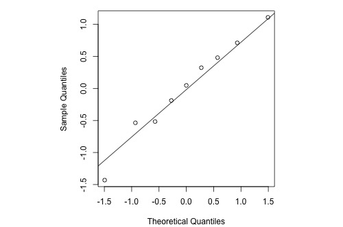
The diagonal line (which passes through the lower and upper quartiles of the theoretical distribution) provides a visual assist to assist assess whether the relationship between the theoretical and sample percentiles is linear.

Note that the relationship between the theoretical percentiles and the sample percentiles is approximately linear. Therefore, the normal probability plot of the residuals suggests that the error terms are indeed normally distributed.

Statistical software sometimes provides normality tests to complement the visual assessment available in a normal probability plot (we'll revisit normality tests in Lesson 7). Different software packages sometimes switch the axes for this plot, but its interpretation remains the same.

Let'south take a look at examples of the different kinds of normal probability plots we tin obtain and learn what each tells us.

Source: https://online.stat.psu.edu/stat501/lesson/4/4.6

Posted by: barnescamonwarld1947.blogspot.com

Share this post